Exercise 3, analyzing the Baltic Sea#
import matplotlib.pyplot as plt
import xarray as xr
ds = xr.open_dataset("data/ocean_day3d.nc")
---------------------------------------------------------------------------
KeyError                                  Traceback (most recent call last)
File ~/miniconda3/envs/xarray/lib/python3.10/site-packages/xarray/backends/file_manager.py:199, in CachingFileManager._acquire_with_cache_info(self, needs_lock)
    198 try:
--> 199     file = self._cache[self._key]
    200 except KeyError:

File ~/miniconda3/envs/xarray/lib/python3.10/site-packages/xarray/backends/lru_cache.py:53, in LRUCache.__getitem__(self, key)
     52 with self._lock:
---> 53     value = self._cache[key]
     54     self._cache.move_to_end(key)

KeyError: [<class 'netCDF4._netCDF4.Dataset'>, ('/Users/boergel/Documents/work/climateoftheocean/data/ocean_day3d.nc',), 'r', (('clobber', True), ('diskless', False), ('format', 'NETCDF4'), ('persist', False))]

During handling of the above exception, another exception occurred:

FileNotFoundError                         Traceback (most recent call last)
/Users/boergel/Documents/work/climateoftheocean/2022-01-20-climate-of-the-ocean-h3.ipynb Zelle 3 in <cell line: 1>()
----> <a href='vscode-notebook-cell:/Users/boergel/Documents/work/climateoftheocean/2022-01-20-climate-of-the-ocean-h3.ipynb#W2sZmlsZQ%3D%3D?line=0'>1</a> ds = xr.open_dataset("data/ocean_day3d.nc")

File ~/miniconda3/envs/xarray/lib/python3.10/site-packages/xarray/backends/api.py:495, in open_dataset(filename_or_obj, engine, chunks, cache, decode_cf, mask_and_scale, decode_times, decode_timedelta, use_cftime, concat_characters, decode_coords, drop_variables, backend_kwargs, *args, **kwargs)
    483 decoders = _resolve_decoders_kwargs(
    484     decode_cf,
    485     open_backend_dataset_parameters=backend.open_dataset_parameters,
   (...)
    491     decode_coords=decode_coords,
    492 )
    494 overwrite_encoded_chunks = kwargs.pop("overwrite_encoded_chunks", None)
--> 495 backend_ds = backend.open_dataset(
    496     filename_or_obj,
    497     drop_variables=drop_variables,
    498     **decoders,
    499     **kwargs,
    500 )
    501 ds = _dataset_from_backend_dataset(
    502     backend_ds,
    503     filename_or_obj,
   (...)
    510     **kwargs,
    511 )
    512 return ds

File ~/miniconda3/envs/xarray/lib/python3.10/site-packages/xarray/backends/netCDF4_.py:550, in NetCDF4BackendEntrypoint.open_dataset(self, filename_or_obj, mask_and_scale, decode_times, concat_characters, decode_coords, drop_variables, use_cftime, decode_timedelta, group, mode, format, clobber, diskless, persist, lock, autoclose)
    529 def open_dataset(
    530     self,
    531     filename_or_obj,
   (...)
    546     autoclose=False,
    547 ):
    549     filename_or_obj = _normalize_path(filename_or_obj)
--> 550     store = NetCDF4DataStore.open(
    551         filename_or_obj,
    552         mode=mode,
    553         format=format,
    554         group=group,
    555         clobber=clobber,
    556         diskless=diskless,
    557         persist=persist,
    558         lock=lock,
    559         autoclose=autoclose,
    560     )
    562     store_entrypoint = StoreBackendEntrypoint()
    563     with close_on_error(store):

File ~/miniconda3/envs/xarray/lib/python3.10/site-packages/xarray/backends/netCDF4_.py:379, in NetCDF4DataStore.open(cls, filename, mode, format, group, clobber, diskless, persist, lock, lock_maker, autoclose)
    373 kwargs = dict(
    374     clobber=clobber, diskless=diskless, persist=persist, format=format
    375 )
    376 manager = CachingFileManager(
    377     netCDF4.Dataset, filename, mode=mode, kwargs=kwargs
    378 )
--> 379 return cls(manager, group=group, mode=mode, lock=lock, autoclose=autoclose)

File ~/miniconda3/envs/xarray/lib/python3.10/site-packages/xarray/backends/netCDF4_.py:327, in NetCDF4DataStore.__init__(self, manager, group, mode, lock, autoclose)
    325 self._group = group
    326 self._mode = mode
--> 327 self.format = self.ds.data_model
    328 self._filename = self.ds.filepath()
    329 self.is_remote = is_remote_uri(self._filename)

File ~/miniconda3/envs/xarray/lib/python3.10/site-packages/xarray/backends/netCDF4_.py:388, in NetCDF4DataStore.ds(self)
    386 @property
    387 def ds(self):
--> 388     return self._acquire()

File ~/miniconda3/envs/xarray/lib/python3.10/site-packages/xarray/backends/netCDF4_.py:382, in NetCDF4DataStore._acquire(self, needs_lock)
    381 def _acquire(self, needs_lock=True):
--> 382     with self._manager.acquire_context(needs_lock) as root:
    383         ds = _nc4_require_group(root, self._group, self._mode)
    384     return ds

File ~/miniconda3/envs/xarray/lib/python3.10/contextlib.py:135, in _GeneratorContextManager.__enter__(self)
    133 del self.args, self.kwds, self.func
    134 try:
--> 135     return next(self.gen)
    136 except StopIteration:
    137     raise RuntimeError("generator didn't yield") from None

File ~/miniconda3/envs/xarray/lib/python3.10/site-packages/xarray/backends/file_manager.py:187, in CachingFileManager.acquire_context(self, needs_lock)
    184 @contextlib.contextmanager
    185 def acquire_context(self, needs_lock=True):
    186     """Context manager for acquiring a file."""
--> 187     file, cached = self._acquire_with_cache_info(needs_lock)
    188     try:
    189         yield file

File ~/miniconda3/envs/xarray/lib/python3.10/site-packages/xarray/backends/file_manager.py:205, in CachingFileManager._acquire_with_cache_info(self, needs_lock)
    203     kwargs = kwargs.copy()
    204     kwargs["mode"] = self._mode
--> 205 file = self._opener(*self._args, **kwargs)
    206 if self._mode == "w":
    207     # ensure file doesn't get overriden when opened again
    208     self._mode = "a"

File src/netCDF4/_netCDF4.pyx:2353, in netCDF4._netCDF4.Dataset.__init__()

File src/netCDF4/_netCDF4.pyx:1963, in netCDF4._netCDF4._ensure_nc_success()

FileNotFoundError: [Errno 2] No such file or directory: b'/Users/boergel/Documents/work/climateoftheocean/data/ocean_day3d.nc'
When you start your work at IOW you will start by reading literature about the dynamics of the Baltic Sea. Soon you will notice that nearly every article starts with a paragraph similar to:
“The hydrography of the Baltic Sea depends on the water exchange with the world ocean which is restricted by the narrows and sills of the Danish Straits and on river runoff into the Baltic [Meier and Kauker, 2003].”
Look at this figure (Meier and Kauker, 2003) and zoom on the connection between the world ocean and the Baltic Sea.
The coordinates are : lon=8-17, lat=53-59

Check you data first. In MOM we use different names for lon, lat and depth:
lon = xt_ocean lat = yt_ocean depth = st_ocean
xarray allows you to select areas using
ds.sel(xt_ocean=slice(lon1, lon2), yt_ocean=slice(lat1, lat2))
ds.dims
Frozen({'xt_ocean': 91, 'yt_ocean': 102, 'time': 11, 'nv': 2, 'xu_ocean': 91, 'yu_ocean': 102, 'st_ocean': 100, 'st_edges_ocean': 101, 'sw_ocean': 100, 'sw_edges_ocean': 101})
danish_straits = ds.sel(xt_ocean=slice(,), yt_ocean=slice(,))
# Instead of selecting coordinate, we can also use
# index selction using .isel
# we are selecting the surface and the first timestep of
# the variable salt and plot it

danish_straits.salt.isel(st_ocean=0, time = 0).plot()
<matplotlib.collections.QuadMesh at 0x7fafbf7ec110>
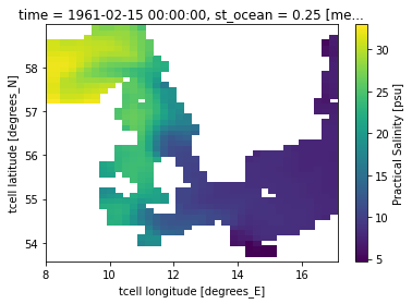
Question 1: What is the first thing you notice, when you compare to the realistic bathymetry above?
Answer:
Question 2: Look at the colobar. What role play the Danish Straits for the salinity of the Baltic Sea?
Answer:
Following on common Baltic Sea introductions, you will find something similar to:
The inflow of freshwater by river runoff and a positive net precipitation cause a positive water balance with respect to the North Sea. The positive water balance leads to strong gradients in salinity and ecosystem variables (Reckermann et al., 2008).
So let’s look at the mean surface salinity!
level = [0,2,4,6,8,10,15,20,30,35]

f, ax = plt.subplots(1)

ds.salt.isel(st_ocean=0).mean("time").plot(levels=level, cmap=plt.cm.jet)
<matplotlib.collections.QuadMesh at 0x7faf43e89090>
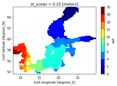
Following Markus second sentence of his paper,
In the long-term mean, high-saline water from the Kattegat enters the Baltic proper and low-saline water leaves the Baltic because of the freshwater surplus.
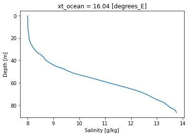
Think about the exchange flow of the Baltic Sea. How would the profile of a transect a 16°E look like?
# We first select the latitude range 53-57, then longitude at 16°E
# note that by using `method="nearest"` we will search for the nearest lon coordinate to 13

transect = ds.sel(yt_ocean=slice(53, 57)).sel(xt_ocean=16, method="nearest")
This leaves us with the dimensions: time, depth and latitude
transect.salt.dims
('time', 'st_ocean', 'yt_ocean')
Markus talks about the long-term mean in his paper. So start by averaging over the time dimension.
using
.mean("time")
transect_mean_time = transect.mean("time")
Now we can average over the latitude, to give us a depth profile.
transect_mean_time_latitude = transect_mean_time.mean("yt_ocean")
f, ax = plt.subplots(1)
transect_mean_time_latitude.salt.plot(ax=ax, y="st_ocean")
ax.set_ylabel("Depth [m]")
ax.set_xlabel("Salinity [g/kg]")
ax.invert_yaxis()
Following along with Markus Paper:
The bottom water in the deep subbasins is ventilated mainly by large perturbations, so-called major Baltic saltwater inflows [Matthäus and Franck, 1992; Fischer and Matthäus, 1996].
In this year we have no strong inflow. However, we can notice inflows of high saline water analyzing the station located in the Arkona Basin.
by2 = ds.sel(xt_ocean = 16.2, yt_ocean = 55.5, method="nearest")
g = (by2.salt - by2.salt.mean("time")).plot(col="time", col_wrap = 3, y="st_ocean")

for ax in g.axes[0]:
    ax.invert_yaxis()
    ax.set_xlabel("Salinity[g/kg]")
    ax.set_ylabel("Depth [m]")

g.fig.tight_layout()
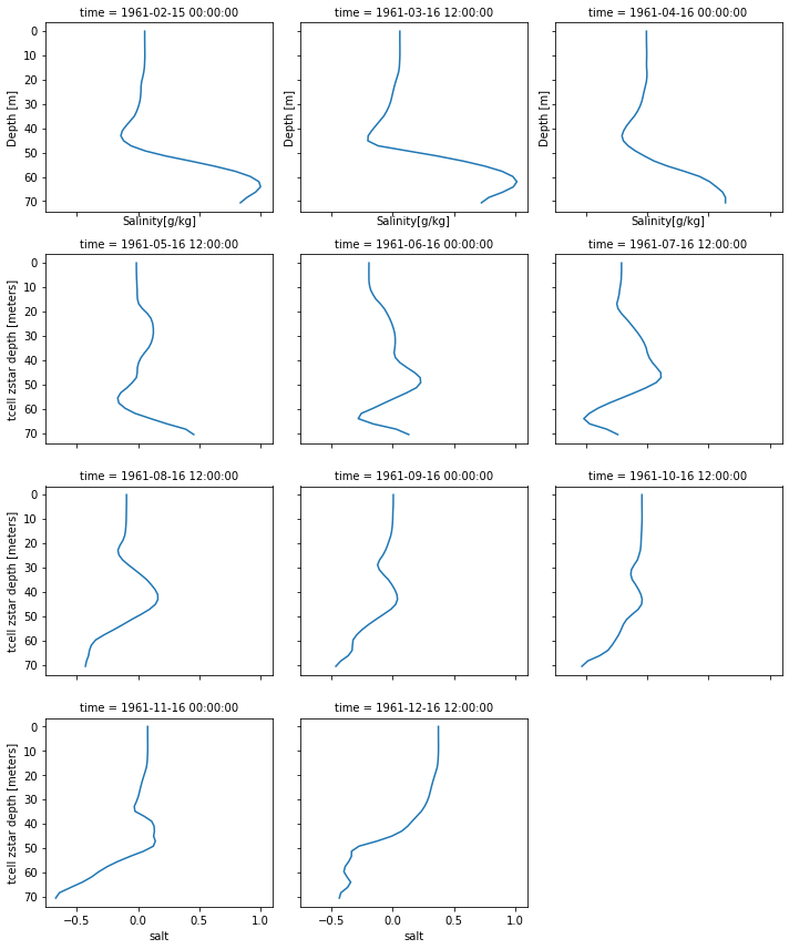
Question 3: Focus on the month of February. What is happening?
These saline inflows are important for the oxygen supply of the deeper layers, since due to the strong stratification in the Baltic Sea only layers above the permanent halocline are directly influenced by the atmosphere and therefore supplied with oxygen (Mohrholz et al., 2015).
Seasonal cycle of the temperature#
We will now look at the depth-averaged seasonal cycle of the Baltic Sea.
ds_temp_season = ds.temp.resample(time="1M").mean("time").mean("st_ocean")
(ds_temp_season-ds_temp_season.mean("time")).plot(col="time", col_wrap =3)
---------------------------------------------------------------------------
NameError                                 Traceback (most recent call last)
/Users/boergel/Documents/work/climateoftheocean/2022-01-20-climate-of-the-ocean-h3.ipynb Zelle 33 in <cell line: 1>()
----> <a href='vscode-notebook-cell:/Users/boergel/Documents/work/climateoftheocean/2022-01-20-climate-of-the-ocean-h3.ipynb#X44sZmlsZQ%3D%3D?line=0'>1</a> (ds_temp_season-ds_temp_season.mean("time")).plot(col="time", col_wrap =3)

NameError: name 'ds_temp_season' is not defined
Question 4: Above you see the deviation from the mean temperature of the Baltic Sea for every single month. Try to discuss the differences for every month.
Sea Ice#
During winter time parts of the Baltic Sea are covered with sea ice. The sea ice influences the air-sea interaction. Sea ice directly influences temperature, salinity, but also the transfer of momentum into the ocean. The annual ice cover varies from only being present in the Bothnian Bay to a nearly fully covered Baltic Sea. Therefore, the Baltic Sea is exposed to great variation in sea ice cover.
ice = xr.open_dataset("data/ice_day.nc")
Let’s start by analyzing the seasonal sea ice cover.
ice
<xarray.Dataset>
Dimensions:      (xt: 91, xb: 92, yt: 102, yb: 103, time: 11, nv: 2, ct: 5, xv: 91, yv: 102)
Coordinates:
  * xt           (xt) float64 8.12 8.36 8.6 8.84 9.08 ... 29.0 29.24 29.48 29.72
  * xb           (xb) float64 8.0 8.24 8.48 8.72 8.96 ... 29.12 29.36 29.6 29.84
  * yt           (yt) float64 53.64 53.76 53.88 54.0 ... 65.4 65.52 65.64 65.76
  * yb           (yb) float64 53.58 53.7 53.82 53.94 ... 65.46 65.58 65.7 65.82
  * time         (time) object 1961-02-15 00:00:00 ... 1961-12-16 12:00:00
  * nv           (nv) float64 1.0 2.0
  * ct           (ct) float64 0.0 0.1 0.3 0.7 1.1
  * xv           (xv) float64 8.24 8.48 8.72 8.96 9.2 ... 29.12 29.36 29.6 29.84
  * yv           (yv) float64 53.7 53.82 53.94 54.06 ... 65.46 65.58 65.7 65.82
Data variables: (12/26)
    FRAZIL       (time, yt, xt) float32 ...
    CN           (time, ct, yt, xt) float32 ...
    MI           (time, yt, xt) float32 ...
    HI           (time, yt, xt) float32 ...
    HS           (time, yt, xt) float32 ...
    TS           (time, yt, xt) float32 ...
    ...           ...
    EVAP         (time, yt, xt) float32 ...
    RUNOFF       (time, yt, xt) float32 ...
    average_T1   (time) datetime64[ns] 1961-02-01 1961-03-01 ... 1961-12-01
    average_T2   (time) datetime64[ns] 1961-03-01 1961-04-01 ... 1962-01-01
    average_DT   (time) timedelta64[ns] 28 days 31 days ... 30 days 31 days
    time_bounds  (time, nv) timedelta64[ns] 0 days 28 days ... 303 days 334 days
Attributes:
    filename:   ice_day.nc
    title:      ERGOM-MOM510 8 n.m. Baltic Hiresaff 1850-2009
    grid_type:  regular
grid_tile: N/A- xt: 91
- xb: 92
- yt: 102
- yb: 103
- time: 11
- nv: 2
- ct: 5
- xv: 91
- yv: 102
- xt(xt)float648.12 8.36 8.6 ... 29.24 29.48 29.72
- long_name :
- longitude
- units :
- degrees_E
- cartesian_axis :
- X
- edges :
- xb
array([ 8.12, 8.36, 8.6 , 8.84, 9.08, 9.32, 9.56, 9.8 , 10.04, 10.28, 10.52, 10.76, 11. , 11.24, 11.48, 11.72, 11.96, 12.2 , 12.44, 12.68, 12.92, 13.16, 13.4 , 13.64, 13.88, 14.12, 14.36, 14.6 , 14.84, 15.08, 15.32, 15.56, 15.8 , 16.04, 16.28, 16.52, 16.76, 17. , 17.24, 17.48, 17.72, 17.96, 18.2 , 18.44, 18.68, 18.92, 19.16, 19.4 , 19.64, 19.88, 20.12, 20.36, 20.6 , 20.84, 21.08, 21.32, 21.56, 21.8 , 22.04, 22.28, 22.52, 22.76, 23. , 23.24, 23.48, 23.72, 23.96, 24.2 , 24.44, 24.68, 24.92, 25.16, 25.4 , 25.64, 25.88, 26.12, 26.36, 26.6 , 26.84, 27.08, 27.32, 27.56, 27.8 , 28.04, 28.28, 28.52, 28.76, 29. , 29.24, 29.48, 29.72]) - xb(xb)float648.0 8.24 8.48 ... 29.36 29.6 29.84
- long_name :
- longitude
- units :
- degrees_E
- cartesian_axis :
- X
array([ 8. , 8.24, 8.48, 8.72, 8.96, 9.2 , 9.44, 9.68, 9.92, 10.16, 10.4 , 10.64, 10.88, 11.12, 11.36, 11.6 , 11.84, 12.08, 12.32, 12.56, 12.8 , 13.04, 13.28, 13.52, 13.76, 14. , 14.24, 14.48, 14.72, 14.96, 15.2 , 15.44, 15.68, 15.92, 16.16, 16.4 , 16.64, 16.88, 17.12, 17.36, 17.6 , 17.84, 18.08, 18.32, 18.56, 18.8 , 19.04, 19.28, 19.52, 19.76, 20. , 20.24, 20.48, 20.72, 20.96, 21.2 , 21.44, 21.68, 21.92, 22.16, 22.4 , 22.64, 22.88, 23.12, 23.36, 23.6 , 23.84, 24.08, 24.32, 24.56, 24.8 , 25.04, 25.28, 25.52, 25.76, 26. , 26.24, 26.48, 26.72, 26.96, 27.2 , 27.44, 27.68, 27.92, 28.16, 28.4 , 28.64, 28.88, 29.12, 29.36, 29.6 , 29.84]) - yt(yt)float6453.64 53.76 53.88 ... 65.64 65.76
- long_name :
- latitude
- units :
- degrees_N
- cartesian_axis :
- Y
- edges :
- yb
array([53.64, 53.76, 53.88, 54. , 54.12, 54.24, 54.36, 54.48, 54.6 , 54.72, 54.84, 54.96, 55.08, 55.2 , 55.32, 55.44, 55.56, 55.68, 55.8 , 55.92, 56.04, 56.16, 56.28, 56.4 , 56.52, 56.64, 56.76, 56.88, 57. , 57.12, 57.24, 57.36, 57.48, 57.6 , 57.72, 57.84, 57.96, 58.08, 58.2 , 58.32, 58.44, 58.56, 58.68, 58.8 , 58.92, 59.04, 59.16, 59.28, 59.4 , 59.52, 59.64, 59.76, 59.88, 60. , 60.12, 60.24, 60.36, 60.48, 60.6 , 60.72, 60.84, 60.96, 61.08, 61.2 , 61.32, 61.44, 61.56, 61.68, 61.8 , 61.92, 62.04, 62.16, 62.28, 62.4 , 62.52, 62.64, 62.76, 62.88, 63. , 63.12, 63.24, 63.36, 63.48, 63.6 , 63.72, 63.84, 63.96, 64.08, 64.2 , 64.32, 64.44, 64.56, 64.68, 64.8 , 64.92, 65.04, 65.16, 65.28, 65.4 , 65.52, 65.64, 65.76]) - yb(yb)float6453.58 53.7 53.82 ... 65.7 65.82
- long_name :
- latitude
- units :
- degrees_N
- cartesian_axis :
- Y
array([53.58, 53.7 , 53.82, 53.94, 54.06, 54.18, 54.3 , 54.42, 54.54, 54.66, 54.78, 54.9 , 55.02, 55.14, 55.26, 55.38, 55.5 , 55.62, 55.74, 55.86, 55.98, 56.1 , 56.22, 56.34, 56.46, 56.58, 56.7 , 56.82, 56.94, 57.06, 57.18, 57.3 , 57.42, 57.54, 57.66, 57.78, 57.9 , 58.02, 58.14, 58.26, 58.38, 58.5 , 58.62, 58.74, 58.86, 58.98, 59.1 , 59.22, 59.34, 59.46, 59.58, 59.7 , 59.82, 59.94, 60.06, 60.18, 60.3 , 60.42, 60.54, 60.66, 60.78, 60.9 , 61.02, 61.14, 61.26, 61.38, 61.5 , 61.62, 61.74, 61.86, 61.98, 62.1 , 62.22, 62.34, 62.46, 62.58, 62.7 , 62.82, 62.94, 63.06, 63.18, 63.3 , 63.42, 63.54, 63.66, 63.78, 63.9 , 64.02, 64.14, 64.26, 64.38, 64.5 , 64.62, 64.74, 64.86, 64.98, 65.1 , 65.22, 65.34, 65.46, 65.58, 65.7 , 65.82]) - time(time)object1961-02-15 00:00:00 ... 1961-12-...
- long_name :
- time
- cartesian_axis :
- T
- calendar_type :
- JULIAN
- bounds :
- time_bounds
array([cftime.DatetimeJulian(1961, 2, 15, 0, 0, 0, 0), cftime.DatetimeJulian(1961, 3, 16, 12, 0, 0, 0), cftime.DatetimeJulian(1961, 4, 16, 0, 0, 0, 0), cftime.DatetimeJulian(1961, 5, 16, 12, 0, 0, 0), cftime.DatetimeJulian(1961, 6, 16, 0, 0, 0, 0), cftime.DatetimeJulian(1961, 7, 16, 12, 0, 0, 0), cftime.DatetimeJulian(1961, 8, 16, 12, 0, 0, 0), cftime.DatetimeJulian(1961, 9, 16, 0, 0, 0, 0), cftime.DatetimeJulian(1961, 10, 16, 12, 0, 0, 0), cftime.DatetimeJulian(1961, 11, 16, 0, 0, 0, 0), cftime.DatetimeJulian(1961, 12, 16, 12, 0, 0, 0)], dtype=object) - nv(nv)float641.0 2.0
- long_name :
- vertex number
- units :
- none
- cartesian_axis :
- N
array([1., 2.])
- ct(ct)float640.0 0.1 0.3 0.7 1.1
- long_name :
- thickness
- units :
- meters
- cartesian_axis :
- Z
array([0. , 0.1, 0.3, 0.7, 1.1])
- xv(xv)float648.24 8.48 8.72 ... 29.36 29.6 29.84
- long_name :
- longitude
- units :
- degrees_E
- cartesian_axis :
- X
array([ 8.24, 8.48, 8.72, 8.96, 9.2 , 9.44, 9.68, 9.92, 10.16, 10.4 , 10.64, 10.88, 11.12, 11.36, 11.6 , 11.84, 12.08, 12.32, 12.56, 12.8 , 13.04, 13.28, 13.52, 13.76, 14. , 14.24, 14.48, 14.72, 14.96, 15.2 , 15.44, 15.68, 15.92, 16.16, 16.4 , 16.64, 16.88, 17.12, 17.36, 17.6 , 17.84, 18.08, 18.32, 18.56, 18.8 , 19.04, 19.28, 19.52, 19.76, 20. , 20.24, 20.48, 20.72, 20.96, 21.2 , 21.44, 21.68, 21.92, 22.16, 22.4 , 22.64, 22.88, 23.12, 23.36, 23.6 , 23.84, 24.08, 24.32, 24.56, 24.8 , 25.04, 25.28, 25.52, 25.76, 26. , 26.24, 26.48, 26.72, 26.96, 27.2 , 27.44, 27.68, 27.92, 28.16, 28.4 , 28.64, 28.88, 29.12, 29.36, 29.6 , 29.84]) - yv(yv)float6453.7 53.82 53.94 ... 65.7 65.82
- long_name :
- latitude
- units :
- degrees_N
- cartesian_axis :
- Y
array([53.7 , 53.82, 53.94, 54.06, 54.18, 54.3 , 54.42, 54.54, 54.66, 54.78,
       54.9 , 55.02, 55.14, 55.26, 55.38, 55.5 , 55.62, 55.74, 55.86, 55.98,
       56.1 , 56.22, 56.34, 56.46, 56.58, 56.7 , 56.82, 56.94, 57.06, 57.18,
       57.3 , 57.42, 57.54, 57.66, 57.78, 57.9 , 58.02, 58.14, 58.26, 58.38,
       58.5 , 58.62, 58.74, 58.86, 58.98, 59.1 , 59.22, 59.34, 59.46, 59.58,
       59.7 , 59.82, 59.94, 60.06, 60.18, 60.3 , 60.42, 60.54, 60.66, 60.78,
       60.9 , 61.02, 61.14, 61.26, 61.38, 61.5 , 61.62, 61.74, 61.86, 61.98,
       62.1 , 62.22, 62.34, 62.46, 62.58, 62.7 , 62.82, 62.94, 63.06, 63.18,
       63.3 , 63.42, 63.54, 63.66, 63.78, 63.9 , 64.02, 64.14, 64.26, 64.38,
       64.5 , 64.62, 64.74, 64.86, 64.98, 65.1 , 65.22, 65.34, 65.46, 65.58,
       65.7 , 65.82])
- FRAZIL(time, yt, xt)float32...
- long_name :
- energy flux of frazil formation
- units :
- W/m^2
- cell_methods :
- time: mean
- time_avg_info :
- average_T1,average_T2,average_DT
[102102 values with dtype=float32]
- CN(time, ct, yt, xt)float32...
- long_name :
- ice concentration
- units :
- 0-1
- cell_methods :
- time: mean
- time_avg_info :
- average_T1,average_T2,average_DT
[510510 values with dtype=float32]
- MI(time, yt, xt)float32...
- long_name :
- ice mass
- units :
- kg/m^2
- cell_methods :
- time: mean
- time_avg_info :
- average_T1,average_T2,average_DT
[102102 values with dtype=float32]
- HI(time, yt, xt)float32...
- long_name :
- ice thickness
- units :
- m-ice
- cell_methods :
- time: mean
- time_avg_info :
- average_T1,average_T2,average_DT
[102102 values with dtype=float32]
- HS(time, yt, xt)float32...
- long_name :
- snow thickness
- units :
- m-snow
- cell_methods :
- time: mean
- time_avg_info :
- average_T1,average_T2,average_DT
[102102 values with dtype=float32]
- TS(time, yt, xt)float32...
- long_name :
- surface temperature
- units :
- C
- cell_methods :
- time: mean
- time_avg_info :
- average_T1,average_T2,average_DT
[102102 values with dtype=float32]
- T1(time, yt, xt)float32...
- long_name :
- upper ice layer temperature
- units :
- C
- cell_methods :
- time: mean
- time_avg_info :
- average_T1,average_T2,average_DT
[102102 values with dtype=float32]
- T2(time, yt, xt)float32...
- long_name :
- lower ice layer temperature
- units :
- C
- cell_methods :
- time: mean
- time_avg_info :
- average_T1,average_T2,average_DT
[102102 values with dtype=float32]
- ALB(time, yt, xt)float32...
- long_name :
- surface albedo
- units :
- 0-1
- cell_methods :
- time: mean
- time_avg_info :
- average_T1,average_T2,average_DT
[102102 values with dtype=float32]
- SW(time, yt, xt)float32...
- long_name :
- short wave heat flux
- units :
- W/m^2
- cell_methods :
- time: mean
- time_avg_info :
- average_T1,average_T2,average_DT
[102102 values with dtype=float32]
- LW(time, yt, xt)float32...
- long_name :
- long wave heat flux over ice
- units :
- W/m^2
- cell_methods :
- time: mean
- time_avg_info :
- average_T1,average_T2,average_DT
[102102 values with dtype=float32]
- TMELT(time, yt, xt)float32...
- long_name :
- upper surface melting energy flux
- units :
- W/m^2
- cell_methods :
- time: mean
- time_avg_info :
- average_T1,average_T2,average_DT
[102102 values with dtype=float32]
- BMELT(time, yt, xt)float32...
- long_name :
- bottom surface melting energy flux
- units :
- W/m^2
- cell_methods :
- time: mean
- time_avg_info :
- average_T1,average_T2,average_DT
[102102 values with dtype=float32]
- UI(time, yv, xv)float32...
- long_name :
- ice velocity - x component
- units :
- m/s
- cell_methods :
- time: mean
- time_avg_info :
- average_T1,average_T2,average_DT
[102102 values with dtype=float32]
- VI(time, yv, xv)float32...
- long_name :
- ice velocity - y component
- units :
- m/s
- cell_methods :
- time: mean
- time_avg_info :
- average_T1,average_T2,average_DT
[102102 values with dtype=float32]
- SLP(time, yt, xt)float32...
- long_name :
- sea level pressure
- units :
- Pa
- cell_methods :
- time: mean
- time_avg_info :
- average_T1,average_T2,average_DT
[102102 values with dtype=float32]
- SST(time, yt, xt)float32...
- long_name :
- sea surface temperature
- units :
- deg-C
- cell_methods :
- time: mean
- time_avg_info :
- average_T1,average_T2,average_DT
[102102 values with dtype=float32]
- SSS(time, yt, xt)float32...
- long_name :
- sea surface salinity
- units :
- psu
- cell_methods :
- time: mean
- time_avg_info :
- average_T1,average_T2,average_DT
[102102 values with dtype=float32]
- SNOWFL(time, yt, xt)float32...
- long_name :
- rate of snow fall
- units :
- kg/(m^2*s)
- cell_methods :
- time: mean
- time_avg_info :
- average_T1,average_T2,average_DT
[102102 values with dtype=float32]
- RAIN(time, yt, xt)float32...
- long_name :
- rate of rain fall
- units :
- kg/(m^2*s)
- cell_methods :
- time: mean
- time_avg_info :
- average_T1,average_T2,average_DT
[102102 values with dtype=float32]
- EVAP(time, yt, xt)float32...
- long_name :
- evaporation
- units :
- kg/(m^2*s)
- cell_methods :
- time: mean
- time_avg_info :
- average_T1,average_T2,average_DT
[102102 values with dtype=float32]
- RUNOFF(time, yt, xt)float32...
- long_name :
- liquid runoff
- units :
- kg/(m^2*s)
- cell_methods :
- time: mean
- time_avg_info :
- average_T1,average_T2,average_DT
[102102 values with dtype=float32]
- average_T1(time)datetime64[ns]...
- long_name :
- Start time for average period
array(['1961-02-01T00:00:00.000000000', '1961-03-01T00:00:00.000000000', '1961-04-01T00:00:00.000000000', '1961-05-01T00:00:00.000000000', '1961-06-01T00:00:00.000000000', '1961-07-01T00:00:00.000000000', '1961-08-01T00:00:00.000000000', '1961-09-01T00:00:00.000000000', '1961-10-01T00:00:00.000000000', '1961-11-01T00:00:00.000000000', '1961-12-01T00:00:00.000000000'], dtype='datetime64[ns]') - average_T2(time)datetime64[ns]...
- long_name :
- End time for average period
array(['1961-03-01T00:00:00.000000000', '1961-04-01T00:00:00.000000000', '1961-05-01T00:00:00.000000000', '1961-06-01T00:00:00.000000000', '1961-07-01T00:00:00.000000000', '1961-08-01T00:00:00.000000000', '1961-09-01T00:00:00.000000000', '1961-10-01T00:00:00.000000000', '1961-11-01T00:00:00.000000000', '1961-12-01T00:00:00.000000000', '1962-01-01T00:00:00.000000000'], dtype='datetime64[ns]') - average_DT(time)timedelta64[ns]...
- long_name :
- Length of average period
array([2419200000000000, 2678400000000000, 2592000000000000, 2678400000000000, 2592000000000000, 2678400000000000, 2678400000000000, 2592000000000000, 2678400000000000, 2592000000000000, 2678400000000000], dtype='timedelta64[ns]') - time_bounds(time, nv)timedelta64[ns]...
- long_name :
- time axis boundaries
- calendar :
- JULIAN
array([[                0,  2419200000000000],
       [ 2419200000000000,  5097600000000000],
       [ 5097600000000000,  7689600000000000],
       [ 7689600000000000, 10368000000000000],
       [10368000000000000, 12960000000000000],
       [12960000000000000, 15638400000000000],
       [15638400000000000, 18316800000000000],
       [18316800000000000, 20908800000000000],
       [20908800000000000, 23587200000000000],
       [23587200000000000, 26179200000000000],
       [26179200000000000, 28857600000000000]], dtype='timedelta64[ns]')
- filename :
- ice_day.nc
- title :
- ERGOM-MOM510 8 n.m. Baltic Hiresaff 1850-2009
- grid_type :
- regular
- grid_tile :
- N/A
ice.MI.resample(time="1M").mean().plot(col="time", col_wrap=4)
<xarray.plot.facetgrid.FacetGrid at 0x7faf3e711f10>
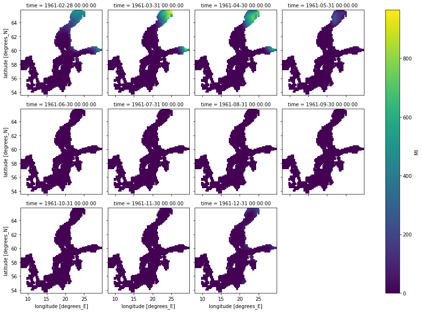
Question 5: Why do we find sea ice in the North but not in the central Baltic Sea?