Lecture 6, Heat transports

Lecture 6, Heat transports#

Two-dimensional advection-diffusion of heat

import xarray as xr
import numpy as np
import matplotlib.pyplot as plt

from ipywidgets import interact, interactive, fixed, interact_manual
import ipywidgets as widgets

from IPython.display import HTML
from IPython.display import display

1) Background: two-dimensional advection-diffusion#

1.1) The two-dimensional advection-diffusion equation#

Recall from the last Lecture that the one-dimensional advection-diffusion equation is written as

\frac{\partial T (x, t)}{\partial t} = - U \frac{\partial T}{\partial x} + κ \frac{\partial^{2} T}{\partial x^{2}},

where $T (x, t)$ is the temperature, $U$ is a constant advective velocity and $κ$ is the diffusivity.

The two-dimensional advection diffusion equation simply adds advection and diffusion operators acting in a second dimensions $y$ (orthogonal to $x$ ).

\frac{\partial T (x, y, t)}{\partial t} = u (x, y) \frac{\partial T}{\partial x} + v (x, y) \frac{\partial T}{\partial y} + κ (\frac{\partial^{2} T}{\partial x^{2}} + \frac{\partial^{2} T}{\partial y^{2}}),

where $\vec{u} (x, y) = (u, v) = u \hat{x} + v \hat{y}$ is a velocity vector field.

Throughout the rest of the Climate Modelling module, we will consider $x$ to be the longitundinal direction (positive from west to east) and $y$ to the be the latitudinal direction (positive from south to north).

1.2) Reminder: Multivariable shorthand notation#

Conventionally, the two-dimensional advection-diffusion equation is written more succintly as

\frac{\partial T (x, y, t)}{\partial t} = - \vec{u} \cdot \nabla T + κ \nabla^{2} T,

using the following shorthand notation.

The gradient operator is defined as

\nabla \equiv (\frac{\partial}{\partial x}, \frac{\partial}{\partial y})

such that

\nabla T = (\frac{\partial T}{\partial x}, \frac{\partial T}{\partial y})

\vec{u} \cdot \nabla T = (u, v) \cdot (\frac{\partial T}{\partial x}, \frac{\partial T}{\partial y}) = u \frac{\partial T}{\partial x} + v \frac{\partial T}{\partial y} .

The Laplacian operator $\nabla^{2}$ (sometimes denoted $Δ$ ) is defined as

\nabla^{2} = \frac{\partial^{2}}{\partial x^{2}} + \frac{\partial^{2}}{\partial y^{2}}

such that

\nabla^{2} T = \frac{\partial^{2} T}{\partial x^{2}} + \frac{\partial^{2} T}{\partial y^{2}} .

The divergence operator is defined as $\nabla \cdot []$ , such that

\nabla \cdot \vec{u} = (\frac{\partial}{\partial x}, \frac{\partial}{\partial x}) \cdot (u, v) = \frac{\partial u}{\partial x} + \frac{\partial v}{\partial y} .

Note: Since seawater is largely incompressible, we can approximate ocean currents as a non-divergent flow, with $\nabla \cdot \vec{u} = \frac{\partial u}{\partial x} + \frac{\partial v}{\partial y} = 0$ . Among other implications, this allows us to write:

\begin{align} \vec{u} \cdot \nabla T&= u\frac{\partial T(x,y,t)}{\partial x} + v\frac{\partial T(x,y,t)}{\partial y}\newline &= u\frac{\partial T}{\partial x} + v\frac{\partial T}{\partial y} + T\left(\frac{\partial u}{\partial x} + \frac{\partial v}{\partial y}\right)\newline &= \left( u\frac{\partial T}{\partial x} + T\frac{\partial u}{\partial x} \right) + \left( v\frac{\partial T}{\partial y} + \frac{\partial v}{\partial y} \right) \newline &= \frac{\partial (uT)}{\partial x} + \frac{\partial (vT)}{\partial y}\newline &= \nabla \cdot (\vec{u}T) \end{align}

using the product rule (separately in both $x$ and $y$ ).

This lets us finally re-write the two-dimensional advection-diffusion equation as:

$\frac{\partial T}{\partial t} = - \nabla \cdot (\vec{u} T) + κ \nabla^{2} T$

which is the form we will use in our numerical algorithm below.

2) Numerical implementation#

2.1) Discretizing advection in two dimensions#

In the last lecture we saw that in one dimension we can discretize a first-partial derivative in space using the centered finite difference

\frac{\partial T (x_{i}, t_{n})}{\partial x} \approx \frac{T_{i + 1}^{n} - T_{i - 1}^{n}}{2 Δ x} .

In two dimensions, we discretize the partial derivative the exact same way, except that we also need to keep track of the cell index $j$ in the $y$ dimension:

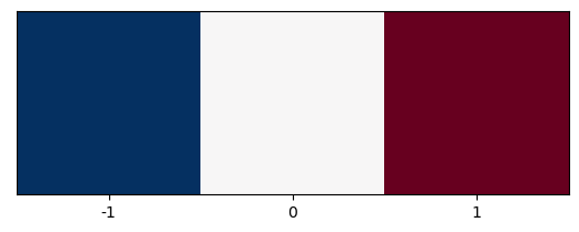
\frac{\partial T (x_{i}, y_{j}, t_{n})}{\partial x} \approx \frac{T_{i + 1, j}^{n} - T_{i - 1, j}^{n}}{2 Δ x} .

The x-gradient kernel below, is shown below, and is reminiscent of the edge-detection or sharpening kernels used in image processing and machine learning:

plt.imshow([[-1,0,1]], cmap=plt.cm.RdBu_r)
plt.xticks([0,1,2], labels=[-1,0,1]);
plt.yticks([]);

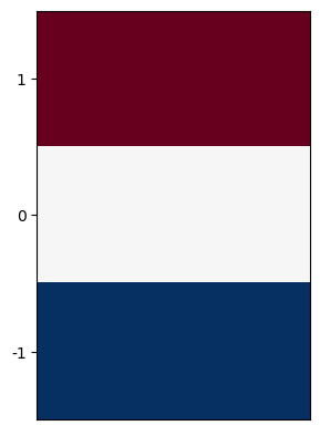
_images/e93d9609d2cd562fb45e769bdbcfb488d51a2149ef026d1007244eb24d0cf720.png

The first-order partial derivative in $y$ is similarly discretized as:

\frac{\partial T (x_{i}, y_{j}, t_{n})}{\partial y} \approx \frac{T_{i, j + 1}^{n} - T_{i, j - 1}^{n}}{2 Δ y} .

Its kernel is shown below.

plt.imshow([[-1,-1],[0,0],[1,1]], cmap=plt.cm.RdBu);
plt.xticks([]);
plt.yticks([0,1,2], labels=[1,0,-1]);

_images/6fab4c80ed51a8f0c1416932e253b22fbfc7ff9a1ca8c78a3a0a939d5134ed8a.png

Now that we have discretized the two derivate terms, we can write out the advective tendency for computing $T_{i, j, n + 1}$ as

u \frac{\partial T}{\partial x} + v \frac{\partial T}{\partial y} \approx u_{i, j}^{n} \frac{T_{i, j + 1}^{n} - T_{i, j - 1}^{n}}{2 Δ y} + v_{i, j}^{n} \frac{T_{i, j + 1}^{n} - T_{i, j - 1}^{n}}{2 Δ y} .

We implement this as a the advect function. This computes the advective tendency for the $(i, j)$ grid cell.

xkernel = np.zeros((1,3))
xkernel[0, :] = np.array([-1,0,1])

ykernel = np.zeros((3,1))
ykernel[:, 0] = np.array([-1,0,1])

class OceanModel:
    
    def __init_(self,T, u, v, deltax, deltay):
        self.T = [T] 
        self.u = u
        self.v = v
        self.deltax = deltax
        self.deltay = deltay
        self.j = np.arange(0, self.T[0].shape[0])
        self.i = np.arange(0, self.T[0].shape[1])
        
    def advect(self, T):
        T_advect = np.zeros((self.j.size, self.i.size))
        
        for j in range(1, T_advect.shape[0] - 1):
            for i in range(1, T_advect.shape[1] - 1):
                T_advect[j, i] = -(self.u[j, i] * np.sum(xkernel[0, :] * T[j, i-1 : i + 2])/(2*self.deltax) +
                                   self.v[j, i] * np.sum(ykernel[:, 0] * T[j-1:j+2, i])/(2*self.deltay))
        return T_advect    

2.2) Discretizing diffusion in two dimensions#

Just as with advection, the process for discretizing the diffusion operators effectively consists of repeating the one-dimensional process for $x$ in a second dimension $y$ , separately:

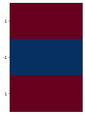
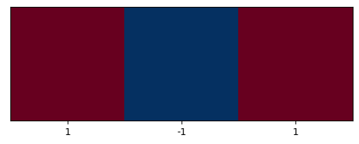
κ (\frac{\partial^{2} T}{\partial x^{2}} + \frac{\partial^{2} T}{\partial y^{2}}) = κ (\frac{T_{i + 1, j}^{n} - 2 T_{i, j}^{n} + T_{i - 1, j}^{n}}{{(Δ x)}^{2}} + \frac{T_{i, j + 1}^{n} - 2 T_{i, j}^{n} + T_{i, j - 1}^{n}}{{(Δ y)}^{2}})

The corresponding $x$ and $y$ second-derivative kernels are shown below:

plt.imshow([[1,1],[0,0],[1,1]], cmap=plt.cm.RdBu_r);
plt.xticks([]);
plt.yticks([0,1,2], labels=[1,-1,1]);

_images/66c8766abd31dc0d723eca861b83032e93c28549bb2436237b6791073623f695.png

plt.imshow([[1,0,1]], cmap=plt.cm.RdBu_r);
plt.xticks([0,1,2], labels=[1,-1,1]);
plt.yticks([]);

_images/e9b5de42a3b12adc55167506dc9f9b804e04bcdbd1cd563b7a5dd4f51d9eba88.png

xkernel_diff = np.zeros((1, 3))
xkernel_diff[0, :] = np.array([1,-2,1])

ykernel_diff = np.zeros((3,1))
ykernel_diff[:, 0] = np.array([1,-2,1])

Just as we did with advection, we implement a diffuse function using multiple dispatch:

class OceanModel():
    
    def __init__(self, T, deltat, windfield, grid, kappa):
        
        self.T = [T]
        self.u = windfield.u
        self.v = windfield.v
        self.deltay = grid.deltay
        self.deltax = grid.deltax
        self.deltat = deltat
        self.kappa = kappa
        self.i = np.arange(0, self.T[0].shape[1])
        self.j = np.arange(0, self.T[0].shape[0])
        self.t = [0]
        self.diffuse_out = []
        self.advect_out = []
        self.t_ = []

    def advect(self, T):
        T_advect = np.zeros((self.j.size, self.i.size))
        for j in range(1, T_advect.shape[0] - 1):
            for i in range(1, T_advect.shape[1] - 1):
                T_advect[j, i] = -(self.u[j, i] * np.sum(xkernel[0, :] * T[j, i-1:i+2])/(2*self.deltax) + \
                                   self.v[j, i] * np.sum(ykernel[:, 0] * T[j-1:j+2, i])/(2*self.deltay))
        return T_advect
                
    def diffuse(self, T):
        T_diffuse= np.zeros((self.j.size, self.i.size))
        for j in range(1, T_diffuse.shape[0] - 1):
            for i in range(1, T_diffuse.shape[1] - 1):
                T_diffuse[j, i] = self.kappa*(np.sum(xkernel_diff[0, :] * T[j, i-1:i+2])/(self.deltax**2) + \
                                              np.sum(ykernel_diff[:, 0] * T[j-1:j+2, i])/(self.deltay**2))      
        return T_diffuse

2.3) No-flux boundary conditions#

We want to impose the no-flux boundary conditions, which states that

$u \frac{\partial T}{\partial x} = κ \frac{\partial T}{\partial x} = 0$ at $x$ boundaries and

$v \frac{\partial T}{\partial y} = κ \frac{\partial T}{\partial y} = 0$ at the $y$ boundaries.

To impose this, we treat $i = 1$ and $i = N_{x}$ as ghost cells, which do not do anything expect help us impose these boundaries conditions. Discretely, the boundary fluxes between $i = 1$ and $i = 2$ vanish if

$\frac{T_{2, j}^{n} - T_{1, j}^{n}}{Δ x} = 0$ or

$T_{1, j}^{n} = T_{2, j}^{n} .$

Thus, we can implement the boundary conditions by updating the temperature of the ghost cells to match their interior-point neighbors:

def update_ghostcells(var):
    var[0, :] = var[1, :];
    var[-1, :] = var[-2, :]
    var[:, 0] = var[:, 1]
    var[:, -1] = var[:, -2]
    return var

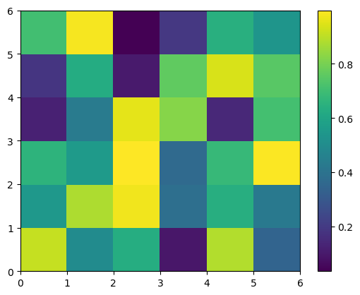
B = np.random.rand(6,6)
plt.pcolor(B)
plt.colorbar()

<matplotlib.colorbar.Colorbar at 0x13330ee00>

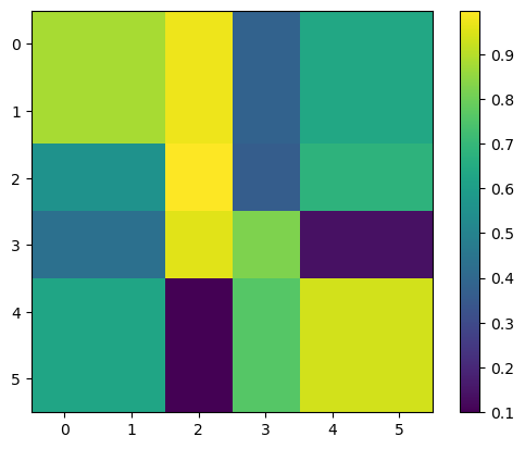
_images/973e758132b5c24e84bb85679198013668acd3fda49c1041af502b846798ca9b.png

B = update_ghostcells(B)

plt.imshow(B)
plt.colorbar()

<matplotlib.colorbar.Colorbar at 0x1333f5660>

_images/d4a86f1fec2de21c9f207e8b327e747934a07e44e4f6dcb33998d81109293bad.png

2.4) Timestepping#

class OceanModel():
    
    def __init__(self, T, deltat, windfield, grid, kappa):
        
        self.T = [T]
        self.u = windfield.u
        self.v = windfield.v
        self.deltay = grid.deltay
        self.deltax = grid.deltax
        self.deltat = deltat
        self.kappa = kappa
        self.i = np.arange(0, self.T[0].shape[1])
        self.j = np.arange(0, self.T[0].shape[0])
        self.t = [0]
        self.diffuse_out = []
        self.advect_out = []
        self.t_ = []

    def advect(self, T):
        T_advect = np.zeros((self.j.size, self.i.size))
        for j in range(1, T_advect.shape[0] - 1):
            for i in range(1, T_advect.shape[1] - 1):
                T_advect[j, i] = -(self.u[j, i] * np.sum(xkernel[0, :] * T[j, i-1:i+2])/(2*self.deltax) + \
                                   self.v[j, i] * np.sum(ykernel[:, 0] * T[j-1:j+2, i])/(2*self.deltax))
        return T_advect
                
    def diffuse(self, T):
        T_diffuse= np.zeros((self.j.size, self.i.size))
        for j in range(1, T_diffuse.shape[0] - 1):
            for i in range(1, T_diffuse.shape[1] - 1):
                T_diffuse[j, i] = self.kappa*(np.sum(xkernel_diff[0, :] * T[j, i-1:i+2])/(self.deltax**2) + \
                                              np.sum(ykernel_diff[:, 0] * T[j-1:j+2, i])/(self.deltay**2))      
        return T_diffuse
    
    def timestep(self):
        T_ = self.T[-1].copy()
        T_ = update_ghostcells(T_)
        tendencies = self.advect(self.T[-1]) + self.diffuse(self.T[-1])
        T_ = self.deltat * tendencies + T_
        self.T.append(T_)
        self.t.append(self.t[-1] + self.deltat)

class grid:   
    """ Creates grid for ocean model
    Args:
    -------
    
    N: Number of grid points (NxN)
    L: Length of domain
    """
    def __init__(self, N, L):
        self.deltax = L / N
        self.deltay = L / N
        self.xs = np.arange(0-self.deltax/2, L+self.deltax/2, self.deltax) 
        self.ys = np.arange(-L-self.deltay/2, L+self.deltay/2, self.deltay)   

        self.N = N
        self.L = L
        self.Nx = len(self.xs)
        self.Ny = len(self.ys)
        self.grid, _= np.meshgrid(self.ys, self.xs, sparse=False, indexing='ij')
        
class windfield:
    """Calculates wind velocity
    
    Args:
    ------
    Grid: class grid()
    option: zero, or single gyre
    
    """
    
    def __init__(self, grid, option = "zero"):
        if option == "zero":
            self.u = np.zeros((grid.grid.shape))
            self.v = np.zeros((grid.grid.shape))
        if option == "single_gyre":
            u, v = PointVortex(grid)
            self.u = u
            self.v = v

Initialize $10 x 10$ grid domain with $L = 6000000 m$ and a windfield, where all velocities are set to zero. This should result in diffusion only.

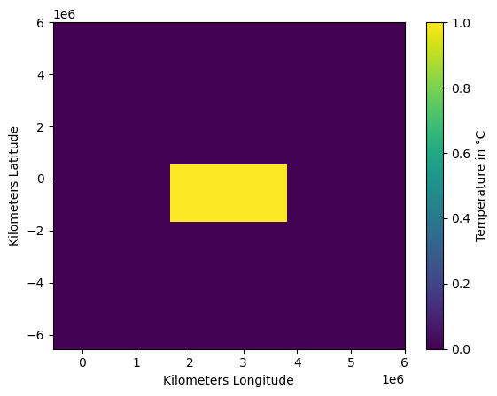
Initialize temperature field with rectangular non-zero box.

my_grid = grid(N = 11, L = 6e6)
my_wind = windfield(my_grid, option = "zero")
my_temp = np.zeros((my_grid.grid.shape)) 
my_temp[9:13, 4:8] = 1

my_grid.grid.shape

(23, 12)

plt.pcolor(my_grid.xs, my_grid.ys, my_temp)
plt.colorbar(label = "Temperature in °C");
plt.ylabel("Kilometers Latitude");
plt.xlabel("Kilometers Longitude");

_images/c32b26f405a54e118653a064262ef6b8f256e7eaac039d78687dd5f6e9b643e1.png

deltat = 12*60*60 # 12 Hours

def plot_func(steps, temp, deltat, windfield, grid, kappa, anomaly = False):
    my_model = OceanModel(T=temp,
                      deltat=deltat, 
                      windfield=windfield, 
                      grid=grid, 
                      kappa = kappa)
    for step in range(steps):
        my_model.timestep()   
    plt.figure(figsize=(8,8))
    lon, lat = np.meshgrid(grid.xs, grid.ys)
    if anomaly == True:
        plt.pcolor(my_grid.xs, my_grid.ys, my_model.T[-1] - my_model.T[-2], cmap = plt.cm.RdBu_r,
                  vmin = -0.001, vmax = 0.001)
    else:
        plt.pcolor(my_grid.xs, my_grid.ys, my_model.T[-1], vmin = 0, vmax = 1)
    plt.quiver(lon, lat, windfield.u, windfield.v)
    plt.colorbar(label = "Temperature in °C");
    plt.ylabel("Kilometers Latitude");
    plt.xlabel("Kilometers Longitude"); 
    plt.title("Time: {} days".format(int(step/2)))
    plt.show()

interact(plot_func, 
         temp = fixed(my_temp),
         deltat = fixed(deltat),
         windfield = fixed(my_wind),
         grid = fixed(my_grid),
         kappa = fixed(1e4),
         anomaly = widgets.Checkbox(description = "Anomaly", value=False),
         steps = widgets.IntSlider(description="Timesteps", value = 2, min = 1, max = 10000, step = 1));

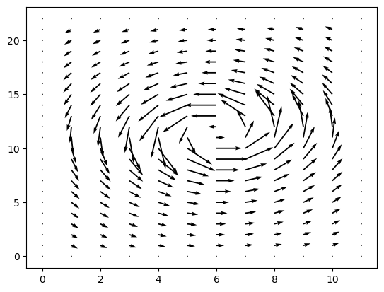
Create single gyre windfield#

def diagnose_velocities(stream, G):    
    dx = np.zeros((G.grid.shape))
    dy = np.zeros((G.grid.shape))
    
    dx = (stream[:, 1:] - stream[:, 0:-1])/G.deltax
    dy = (stream[1:, :] - stream[0:-1, :])/G.deltay
    
    u = np.zeros((G.grid.shape))
    v = np.zeros((G.grid.shape))
    
    u = 0.5*(dy[:, 1:] + dy[:, 0:-1])
    v = -0.5*(dx[1:, :] + dx[0:-1, :])
    
    return u, v

def impose_no_flux(u, v):
    u[0, :]  = 0; v[0, :] = 0;
    u[-1,:]  = 0; v[-1,:] = 0;
    u[:, 0]  = 0; v[:, 0] = 0;
    u[:,-1]  = 0; v[:,-1] = 0;
    
    return u, v

def PointVortex(G, omega = 0.6, a = 0.2, x0=0.5, y0 = 0.):
    x = np.arange(-G.deltax/G.L, 1 + G.deltax / G.L, G.deltax / G.L).reshape(1, -1)
    y = np.arange(-1-G.deltay/G.L, 1+ G.deltay / G.L, G.deltay / G.L).reshape(-1, 1)
        
    r = np.sqrt((y - y0)**2 + (x - x0)**2)
    stream = -omega/4*r**2 
    stream[r > a] =  -omega*a**2/4*(1. + 2*np.log(r[r > a]/a))
    
    u, v =  diagnose_velocities(stream, G)
    u, v = impose_no_flux(u, v) 
    u = u * G.L; v = v * G.L
    return u, v

my_wind = windfield(my_grid, option="single_gyre")
plt.quiver(my_wind.u, my_wind.v)

<matplotlib.quiver.Quiver at 0x134f329b0>

_images/760e93c3756bbdf639c71329fec50734e633f41e624b5f9ea0fa9471f9f277b7.png

my_temp = np.zeros((my_grid.grid.shape)) 
my_temp[8:13, :] = 1

plt.pcolor(my_temp)

<matplotlib.collections.PolyCollection at 0x134f30190>

_images/76e979b96a2c070b30fe2a52ca5fadeb22ae66c6808e30ae01525b3b31c68f66.png

my_model = OceanModel(T=my_temp,
                      deltat=deltat, 
                      windfield=my_wind, 
                      grid=my_grid, 
                      kappa = 1e4)

interact(plot_func, 
         temp = fixed(my_temp),
         deltat = fixed(deltat),
         windfield = fixed(my_wind),
         grid = fixed(my_grid),
         kappa = widgets.IntSlider(description="kappa", value = 1e4, min=1e3, max = 1e5, step = 100),
         anomaly = widgets.Checkbox(description = "Anomaly", value=False),
         steps = widgets.IntSlider(description="Timesteps", value = 1, min = 1, max = 1000, step = 1));

Optional: Create two gyres!